Differential Kinematics

The Kinematics chapter fixed the arm's configuration at a single instant. Motion, however, is the variation of that configuration as time passes. Differential kinematics studies the relationship between the rates of change of the joint angles and the resulting endpoint velocity (and, one derivative further, the endpoint acceleration).

This page builds the relationship up from a concrete two-joint arm and then generalizes it to an arbitrary number of joints, mirroring how the skelarm kinematics code is organized.

1. A two-joint arm

Recall the two-joint arm from the Kinematics chapter — a fixed base link \(l_0\) followed by two movable links of length \(l_1\) and \(l_2\). The figure below revisits it, now with the joint velocities \(\dot{q}_1, \dot{q}_2\) and the resulting endpoint velocity drawn in.

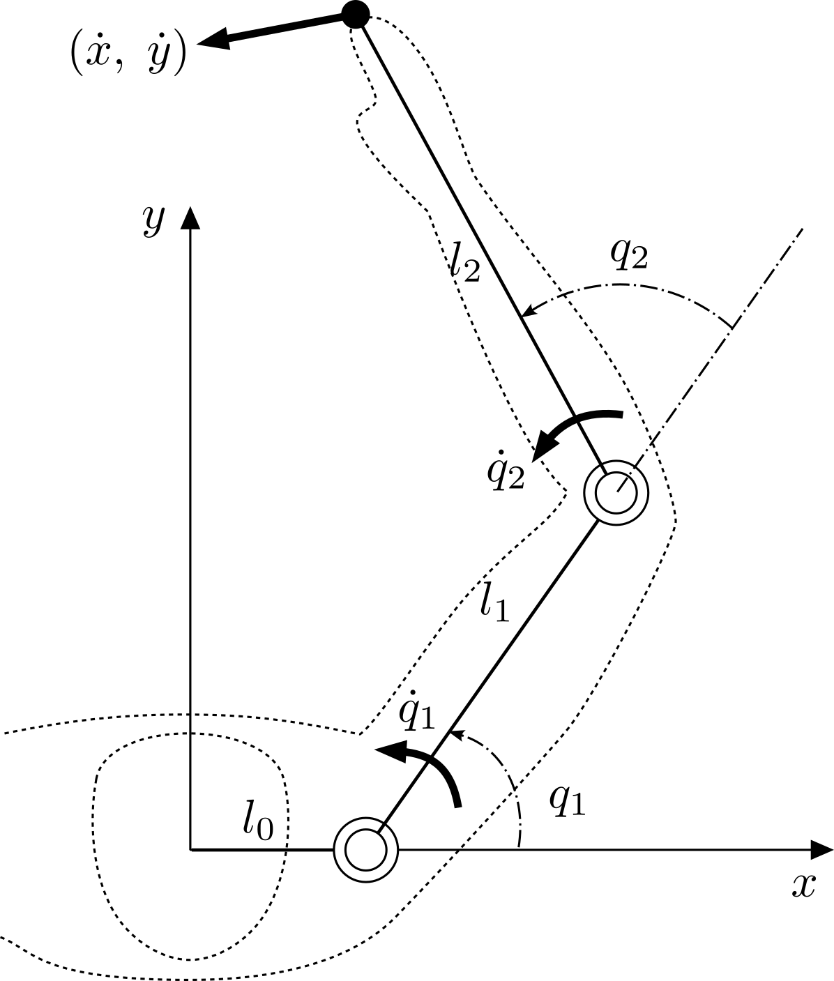
Endpoint velocity of a two-joint arm. The base link \(l_0\) offsets the first joint along the \(x\)-axis; \(q_1, q_2\) are the joint angles and \(\dot{q}_1, \dot{q}_2\) their velocities.

Its endpoint position is

\[ \begin{aligned} x &= l_0 + l_1 \cos q_1 + l_2 \cos(q_1 + q_2) \\ y &= l_1 \sin q_1 + l_2 \sin(q_1 + q_2). \end{aligned} \]

Differentiating with respect to time relates the joint velocities to the endpoint velocity at the current configuration:

\[ \begin{aligned} \dot{x} &= -\dot{q}_1 l_1 \sin q_1 - (\dot{q}_1 + \dot{q}_2) l_2 \sin(q_1 + q_2) \\ \dot{y} &= \dot{q}_1 l_1 \cos q_1 + (\dot{q}_1 + \dot{q}_2) l_2 \cos(q_1 + q_2). \end{aligned} \]

Notice that the constant base length \(l_0\) drops out of the velocity: it shifts where the arm is but never how fast the endpoint moves.

2. Generalizing to \(n\) joints

Introduce the absolute link angle \(\theta_i\) — the orientation of link \(i\) measured from the \(x\)-axis — so that \(\theta_i = \theta_{i-1} + q_i\). With this notation the pattern above extends to an arm of \(n\) movable links by a recursion that sweeps forward from the base (link \(0\)) to the endpoint (link \(n\)).

Symbols used throughout:

• \(q_i\) — joint angle of joint \(i\), relative to the previous link.
• \(\theta_i\) — absolute angle of link \(i\).
• \((x_i, y_i)\) — position of the tip of link \(i\) (equivalently, the origin of joint \(i+1\)).
• \(l_i\) — length of link \(i\), with \(l_0\) the fixed base link.

Velocity

The base link is rigid, so the base of the chain starts from rest:

\[ \dot{\theta}_0 = 0, \qquad \dot{x}_0 = 0, \qquad \dot{y}_0 = 0. \]

(The base length still enters the positions through \(x_0 = l_0\), \(y_0 = 0\), but not the velocities.) For \(i = 1, \dots, n\):

\[ \begin{aligned} \dot{\theta}_i &= \dot{\theta}_{i-1} + \dot{q}_i \\ \dot{x}_i &= \dot{x}_{i-1} - \dot{\theta}_i\, l_i \sin \theta_i \\ \dot{y}_i &= \dot{y}_{i-1} + \dot{\theta}_i\, l_i \cos \theta_i. \end{aligned} \]

Running the recursion to \(i = n\) yields the endpoint velocity.

Acceleration

Differentiating once more gives the matching acceleration recursion, again with \(\ddot{\theta}_0 = \ddot{x}_0 = \ddot{y}_0 = 0\) and, for \(i = 1, \dots, n\):

\[ \begin{aligned} \ddot{\theta}_i &= \ddot{\theta}_{i-1} + \ddot{q}_i \\ \ddot{x}_i &= \ddot{x}_{i-1} - \dot{\theta}_i^2\, l_i \cos \theta_i - \ddot{\theta}_i\, l_i \sin \theta_i \\ \ddot{y}_i &= \ddot{y}_{i-1} - \dot{\theta}_i^2\, l_i \sin \theta_i + \ddot{\theta}_i\, l_i \cos \theta_i. \end{aligned} \]

These two recursions are exactly what compute_forward_kinematics evaluates as it walks the link list; the fixed base link (stored as links[0]) simply contributes its \(l_0\) offset with zero velocity and acceleration.

3. The Jacobian

The endpoint velocity is linear in the joint velocities, so it can be packed into a matrix–vector product. Writing the endpoint as \((x, y) \equiv (x_n, y_n)\),

\[ \begin{bmatrix} \dot{x} \\ \dot{y} \end{bmatrix} = J \dot{q} = \begin{bmatrix} j_{x1} & \cdots & j_{xn} \\ j_{y1} & \cdots & j_{yn} \end{bmatrix} \begin{bmatrix} \dot{q}_1 \\ \vdots \\ \dot{q}_n \end{bmatrix}, \qquad \dot{x} = \sum_{i=1}^{n} j_{xi}\, \dot{q}_i, \quad \dot{y} = \sum_{i=1}^{n} j_{yi}\, \dot{q}_i. \]

The columns \(j_{xi}, j_{yi}\) are the Jacobian basis for joint \(i\). They can be assembled by a backward recursion (from the tip down to joint \(1\), with a virtual zero column at \(n+1\)):

\[ j_{x(n+1)} = 0, \quad j_{xi} = j_{x(i+1)} - l_i \sin \theta_i, \qquad j_{y(n+1)} = 0, \quad j_{yi} = j_{y(i+1)} + l_i \cos \theta_i. \]

Equivalently — and this is the compact form skelarm uses — each column is the lever arm from joint \(i\) to the endpoint, rotated by a quarter turn:

\[ j_{xi} = -(y_n - y_{i-1}), \qquad j_{yi} = x_n - x_{i-1}, \]

where \((x_{i-1}, y_{i-1})\) is the origin of joint \(i\). The two expressions agree, and both equal the partial derivatives of the endpoint position,

\[ j_{xi} = \frac{\partial x}{\partial q_i}, \qquad j_{yi} = \frac{\partial y}{\partial q_i}, \]

which is precisely why \(J = \partial (x, y) / \partial (q_1, \dots, q_n)\).

4. Centripetal and Coriolis basis

Differentiating the Jacobian relation extends the idea to acceleration:

\[ \begin{aligned} \ddot{x} &= \sum_{i=1}^{n} \left( j_{xi}\, \ddot{q}_i + h_{xi}\, \dot{q}_i \right) \\ \ddot{y} &= \sum_{i=1}^{n} \left( j_{yi}\, \ddot{q}_i + h_{yi}\, \dot{q}_i \right), \end{aligned} \]

where \(h_{xi}, h_{yi}\) are the time derivatives of the Jacobian columns, \(h_{xi} = \dot{j}_{xi}\) and \(h_{yi} = \dot{j}_{yi}\). The products \(h_{\ast i}\dot{q}_i\) are the centripetal and Coriolis accelerations, so \(h_{\ast i}\) is called the centripetal/Coriolis basis. Geometrically it is the velocity counterpart of the Jacobian column,

\[ h_{xi} = -(\dot{y}_n - \dot{y}_{i-1}), \qquad h_{yi} = \dot{x}_n - \dot{x}_{i-1}, \]

with \((\dot{x}_{i-1}, \dot{y}_{i-1})\) the velocity of joint \(i\)'s origin.

5. Implementation

The differential-kinematics helpers in skelarm.kinematics make these two viewpoints — the forward recursion and the Jacobian/basis form — independently computable, which is exactly what lets one validate the other.

Function	Returns	Theory
compute_forward_kinematics	(updates link state)	Section 2; forward velocity/acceleration recursion
compute_jacobian	\(2 \times n\) matrix \(J\)	Section 3
compute_coriolis_basis	\(2 \times n\) matrix \(H\)	Section 4
compute_endpoint_velocity	\(J \dot{q}\)	Section 3
compute_endpoint_acceleration	\(J \ddot{q} + H \dot{q}\)	Section 4

The Jacobian helpers read the joint and endpoint state populated by compute_forward_kinematics, so call it first. Because the endpoint velocity and acceleration are then available from two routes — propagated directly by the forward recursion (stored on the tip link as vx, vy, ax, ay) and reconstructed from the Jacobian and basis — comparing them is a built-in consistency check:

import numpy as np
from skelarm import (
    Skeleton, LinkProp,
    compute_forward_kinematics,
    compute_endpoint_velocity, compute_endpoint_acceleration,
)

skeleton = Skeleton(
    [LinkProp(length=1.0, m=1.0, i=0.1, rgx=0.5, rgy=0.0, qmin=-np.pi, qmax=np.pi),
     LinkProp(length=0.8, m=1.0, i=0.1, rgx=0.4, rgy=0.0, qmin=-np.pi, qmax=np.pi)],
    base_length=0.3,
)
skeleton.q = np.array([0.4, -0.7])
skeleton.dq = np.array([0.8, 0.3])
skeleton.ddq = np.array([0.6, -0.4])

compute_forward_kinematics(skeleton)
tip = skeleton.links[-1]

assert np.allclose(compute_endpoint_velocity(skeleton), [tip.vx, tip.vy])
assert np.allclose(compute_endpoint_acceleration(skeleton), [tip.ax, tip.ay])

The base link is set up in the Kinematics chapter; here it contributes only a constant offset, since a fixed link has no velocity.