Trajectory Filtering and Interpolation

A reference trajectory for trajectory-tracking control is often supplied as a finite series of samples \((t_i, y_i)\) — a tip path or a per-joint angle series recorded with tools/trajectory_recorder.py, or generated offline. Two numerical operations turn such a series into a reference the controller can sample at its own rate: smoothing (to suppress measurement/teaching noise before it is amplified by differentiation) and interpolation (to resample between the given times and, for the cubic spline, to obtain smooth derivatives). skelarm implements both from scratch in skelarm.filtering and skelarm.interpolation.

1. Interpolation

Given samples \(y_0, \dots, y_N\) at increasing times \(t_0, \dots, t_N\), an interpolant \(\hat{y}(t)\) passes through every sample, \(\hat{y}(t_i) = y_i\). A multi-column series is interpolated column by column.

Linear

Piecewise-linear interpolation joins consecutive samples with straight lines: on \([t_i, t_{i+1}]\),

\[\hat{y}(t) = y_i + \frac{t - t_i}{t_{i+1} - t_i}\,(y_{i+1} - y_i).\]

It is shape-preserving and never overshoots, but is only \(C^0\) — its derivative is piecewise-constant and discontinuous at the nodes.

Natural cubic spline

A cubic spline is a \(C^2\) piecewise-cubic. Writing the second derivatives at the nodes as \(M_i = \hat{y}''(t_i)\) and \(h_i = t_{i+1} - t_i\), continuity of \(\hat{y}'\) gives the tridiagonal system (for the interior nodes \(i = 1, \dots, N-1\))

\[h_{i-1} M_{i-1} + 2(h_{i-1} + h_i) M_i + h_i M_{i+1} = 6\!\left(\frac{y_{i+1}-y_i}{h_i} - \frac{y_i - y_{i-1}}{h_{i-1}}\right),\]

with the natural boundary conditions \(M_0 = M_N = 0\). skelarm solves it with the Thomas algorithm (Gaussian elimination specialized to a tridiagonal matrix). On \([t_i, t_{i+1}]\), with \(a = (t_{i+1}-t)/h_i\) and \(b = (t-t_i)/h_i\),

\[\hat{y}(t) = a\,y_i + b\,y_{i+1} + \big[(a^3-a) M_i + (b^3-b) M_{i+1}\big]\frac{h_i^2}{6},\]

and the first and second derivatives follow analytically. This makes the cubic spline the right default for deriving smooth velocity \(\dot{q}_r\) and acceleration \(\ddot{q}_r\) references.

Barycentric Lagrange

The unique degree-\(N\) polynomial through all \(N+1\) nodes is evaluated in the stable barycentric form

\[\hat{y}(t) = \frac{\sum_j \dfrac{w_j}{t - t_j}\, y_j}{\sum_j \dfrac{w_j}{t - t_j}}, \qquad w_j = \frac{1}{\prod_{k \neq j}(t_j - t_k)}.\]

It is exact for polynomial data, but a high-degree polynomial through many equally spaced nodes oscillates wildly near the ends (the Runge phenomenon), so reserve it for short series.

The three interpolators compared

examples/interpolation_demo.py reconstructs a known smooth reference from coarse equispaced samples and measures each interpolator against the analytic truth:

uv run python examples/interpolation_demo.py

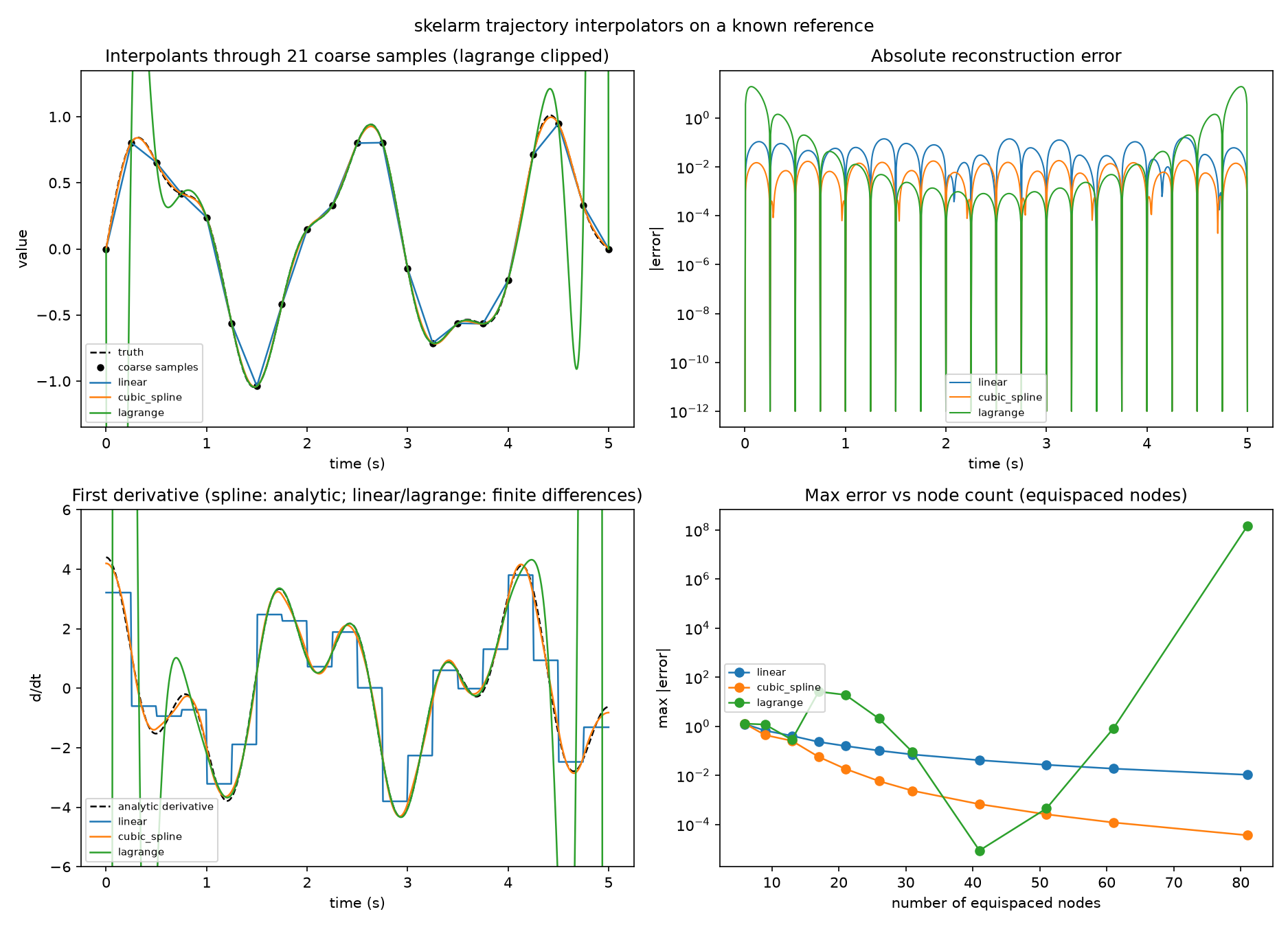
At 21 nodes the cubic spline is roughly seven times more accurate than linear (RMSE 0.009 vs 0.062) — a somewhat favorable case, since this reference happens to have zero endpoint curvature, exactly the natural boundary condition; with nonzero endpoint curvature the margin narrows to about fourfold. The spline's analytic first derivative tracks the true one where linear's finite-difference slope is a staircase. The Lagrange polynomial illustrates the warning above, and the sweep panel shows how untrustworthy a high-degree equispaced fit is: edge oscillations reach absolute errors around 26 at 17 nodes, a transiently tiny error appears near 41 nodes, and beyond roughly 60 nodes the finite-precision evaluation blows up outright (~10⁸ by 81 nodes) — whatever exact arithmetic would promise for an analytic signal, the floating-point implementation does not stay converged.

2. Smoothing filters

A jagged reference (e.g. a hand-taught path) has high-frequency content that differentiation amplifies. A low-pass filter removes content above a cutoff frequency \(f_c\) while preserving the slow motion. The series must be uniformly sampled with period \(\Delta t\); the Nyquist frequency is \(1/(2\Delta t)\). skelarm offers four kinds — two frequency-domain (cutoff-based) and two window-based.

First-order (RC) low-pass

The one-pole filter has the recursion

\[y_i = y_{i-1} + \alpha\,(x_i - y_{i-1}), \qquad \alpha = \frac{\Delta t}{RC + \Delta t}, \quad RC = \frac{1}{2\pi f_c}.\]

It is cheap but rolls off gently (−20 dB/decade).

Butterworth

A Butterworth filter of order \(n\) has a maximally flat passband. Its analog prototype places \(n\) poles evenly on the left half of a circle of radius \(\omega_c\),

\[s_k = \omega_c \exp\!\left(j\,\frac{\pi(2k+1)}{2n} + j\frac{\pi}{2}\right), \qquad k = 0, \dots, n-1,\]

and rolls off at \(-20n\) dB/decade. skelarm maps the analog filter to the discrete domain with the bilinear transform \(s = \frac{2}{\Delta t}\frac{z-1}{z+1}\), pre-warping the cutoff \(\omega_a = \frac{2}{\Delta t}\tan(\pi f_c \Delta t)\) so the digital cutoff lands at \(f_c\), and normalizes the gain to unity at DC.

Moving average

A centered moving average over an odd window of \(W = 2m+1\) samples replaces each point with the mean of its neighbours,

\[y_i = \frac{1}{W} \sum_{k=-m}^{m} x_{i+k}.\]

It is the simplest smoother — a finite (FIR) filter with a symmetric (hence phase-free) rectangular kernel that reproduces constants and linear trends exactly in the interior. It is specified by the window length rather than a cutoff.

Savitzky–Golay

A Savitzky–Golay filter fits a polynomial of degree \(p\) to each sliding window of \(W\) samples by least squares and takes the value of that fit at the window centre. The kernel is the centre row of the pseudo-inverse \(\big(A^\top A\big)^{-1} A^\top\) of the Vandermonde design matrix \(A_{kj} = z_k^{\,j}\) over the offsets \(z = -m, \dots, m\). Because the kernel is symmetric it is phase-free, and because the fit is exact for polynomials up to degree \(p\) it preserves peaks and curvature far better than a plain average while still suppressing noise. It is specified by the window length \(W\) and the polynomial order \(p\) (with \(p < W\)).

Zero-phase application

Any causal IIR filter delays the signal (phase lag), which would bias a tracked trajectory, so each filter is applied in a way that leaves no net delay:

• Butterworth runs forward and then backward (filtfilt): the two passes cancel the phase at the cost of squaring the magnitude response (doubling the roll-off in dB). The signal is first extended at each end by a point reflection about its boundary sample, and each pass starts from steady-state initial conditions, so a constant (DC) signal passes through unchanged and edge transients are suppressed.
• First-order (RC) low-pass also runs forward and then backward, squaring its magnitude response, but without padding: each pass is seeded with its first sample, which likewise preserves a constant signal.
• Moving average and Savitzky–Golay are a single convolution with a symmetric, centered kernel, which is phase-free on its own, so their magnitude response is not squared. The signal is mirrored at each end so the window stays full near the edges.

The four filters compared

examples/filtering_demo.py compares all four kinds at representative settings matched by nominal cutoff / window time scale: the window filters are specified by a window length in seconds, so the settings scale with the sample rate. (The final bandwidths still differ by kind — the two IIR filters run forward and backward, which squares their magnitude responses and pulls the effective −3 dB cutoff below the configured value, furthest for the first-order low-pass; the window filters run once.) On a synthetic signal it reports the RMSE against the known ground truth as a mean over ten noise seeds; on the hand-taught recording shipped in docs/assets/teach.sklog.npz it shows the taught tip path and a zoomed view of its final approach — where the raw pointer quantization is visible — with the filters cutting the tip acceleration RMS four- to eight-fold while deviating only 0.9–1.5 mm RMS from the demonstrated path:

uv run python examples/filtering_demo.py

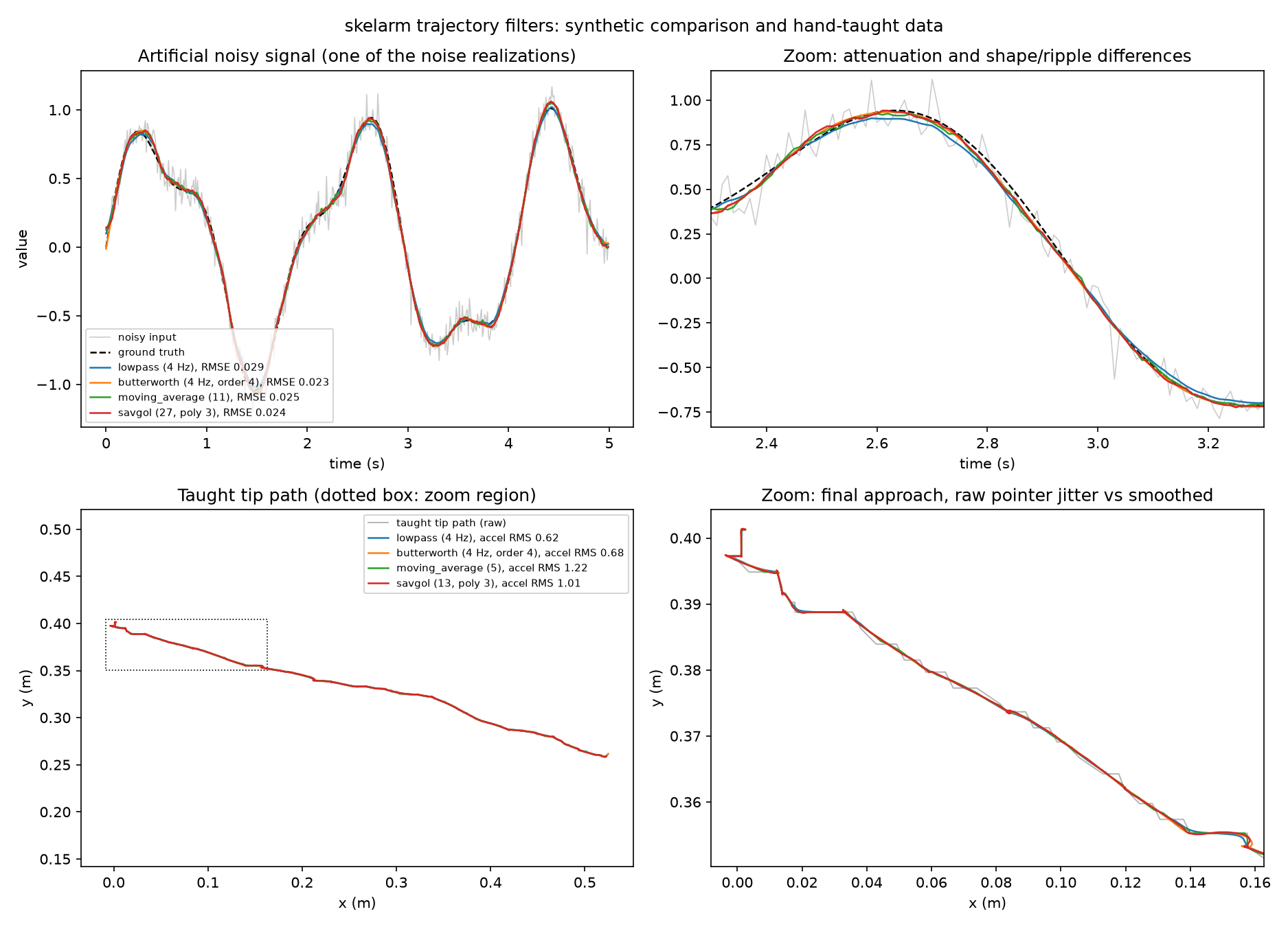
The zoom panels show the characteristic trade-offs: the first-order low-pass attenuates the peak the most for its nominal cutoff, the Butterworth tracks the reference tightest, and Savitzky–Golay preserves curvature well at the cost of a little residual ripple. This is a qualitative comparison of sensible defaults, not a strict ranking — the right choice depends on the reference's frequency content and how much smoothing the task tolerates.

3. How skelarm uses them

The trajectory_tracking and joint_trajectory_tracking task types (Control Configuration) load a reference .sklog.npz, optionally smooth it, then resample_with_derivatives it onto a uniform 20 ms reference grid:

• Task-space (trajectory_tracking): the smoothed tip path becomes a SampledTaskReference, which ik_joint_reference converts to a joint reference.
• Joint-space (joint_trajectory_tracking): the smoothed angle series and its spline derivatives form a SampledJointReference directly (no inverse kinematics).

Controllers read that grid by linear interpolation at every control step, whatever [simulator].dt is, so a finer simulation step does not refine the reference itself.

The filters assume evenly spaced samples. A recorder log is nearly even, but its timestamps are the real elapsed times, so a late timer tick shows up as a longer gap. The series is therefore smoothed as if evenly spaced at its mean sample interval, and the spline is then fitted against the recorded timestamps.